K-Means Land Classification with Dask#
K-Means is a clustering algorithm that creates a segmentation map of different “clusters” which can represent estimated/easily-separable classifications which share similar values to a centroid optimum that represents the groups mean value. The classifications should not be considered accurate and requires verification - however it is a great starting point for unsupervised classification problems to determine separable classes.
For geospatial applications, we can use K-Means to create rough land-classification segmentation maps or generate automated labeled data given supporting methods to verify the classification is correct.
[ ]:
# We will be using Sentinel-2 L2A imagery from Microsoft Planetary Computer STAC server:
!pip install planetary_computer
[ ]:
import os
import rasterio
import rioxarray
import pystac
import stackstac
import datetime
import planetary_computer
import dask
import json
import gcsfs

import dask_ml.cluster

import numpy as np
import xarray as xr
import rioxarray as rxr
import matplotlib.pyplot as plt
import geopandas as gpd

from skimage.exposure import rescale_intensity
from dask_gateway import Gateway
from shapely.geometry import Polygon
from pystac_client import Client
1. Initialize Dask Cluster#
We will use Dask to power our computations of a K-Means algorithm with which will be fitted and used to for predictions. Start by initializing a dask cluster in a separate notebook and connecting to it. We then scaled our cluster to have 3 workers.
Remember to replace the dask cluster’s name below with the one you instantiate.
[4]:
gateway = Gateway()
cluster = gateway.connect('daskhub.81d82a23b4ea4bb2aac199856b4049f2')
client = cluster.get_client()
cluster
AOI#
This AOI was generated from: https://www.keene.edu/campus/maps/tool/
We will, for the purpose of this demonstration, look at the Timberlea suburb in Montreal, Quebec, Canada
[10]:
_polygon = {
  "coordinates": [
    [
      [
        -73.8847303,
        45.4294192
      ],
      [
        -73.883357,
        45.4445361
      ],
      [
        -73.9108229,
        45.4442049
      ],
      [
        -73.9120245,
        45.4263471
      ],
      [
        -73.8847303,
        45.4294192
      ]
    ]
  ],
  "type": "Polygon"
}
[11]:
lon_list = []
lat_list = []

for lon,lat in _polygon['coordinates'][0]:
    lon_list.append(lon)
    lat_list.append(lat)
polygon_geom = Polygon(zip(lon_list, lat_list))
crs = 'EPSG:4326'
polygon = gpd.GeoDataFrame(index=[0], crs=crs, geometry=[polygon_geom])
[12]:
# Set up Stac Client
api = Client.open('https://planetarycomputer.microsoft.com/api/stac/v1')
api
[12]:
Client: microsoft-pc
| id: microsoft-pc |
| title: Microsoft Planetary Computer STAC API |
| description: Searchable spatiotemporal metadata describing Earth science datasets hosted by the Microsoft Planetary Computer |
| type: Catalog |
| conformsTo: ['http://www.opengis.net/spec/cql2/1.0/conf/basic-cql2', 'http://www.opengis.net/spec/cql2/1.0/conf/cql2-json', 'http://www.opengis.net/spec/cql2/1.0/conf/cql2-text', 'http://www.opengis.net/spec/ogcapi-features-1/1.0/conf/core', 'http://www.opengis.net/spec/ogcapi-features-1/1.0/conf/geojson', 'http://www.opengis.net/spec/ogcapi-features-1/1.0/conf/oas30', 'http://www.opengis.net/spec/ogcapi-features-3/1.0/conf/filter', 'https://api.stacspec.org/v1.0.0-rc.1/collections', 'https://api.stacspec.org/v1.0.0-rc.1/core', 'https://api.stacspec.org/v1.0.0-rc.1/item-search', 'https://api.stacspec.org/v1.0.0-rc.1/item-search#fields', 'https://api.stacspec.org/v1.0.0-rc.1/item-search#filter', 'https://api.stacspec.org/v1.0.0-rc.1/item-search#query', 'https://api.stacspec.org/v1.0.0-rc.1/item-search#sort', 'https://api.stacspec.org/v1.0.0-rc.1/ogcapi-features'] |
Children
Only the first child shown
CollectionClient: daymet-annual-pr
| id: daymet-annual-pr |
| title: Daymet Annual Puerto Rico |
| description: Annual climate summaries derived from [Daymet](https://daymet.ornl.gov) Version 4 daily data at a 1 km x 1 km spatial resolution for five variables: minimum and maximum temperature, precipitation, vapor pressure, and snow water equivalent. Annual averages are provided for minimum and maximum temperature, vapor pressure, and snow water equivalent, and annual totals are provided for the precipitation variable. [Daymet](https://daymet.ornl.gov/) provides measurements of near-surface meteorological conditions; the main purpose is to provide data estimates where no instrumentation exists. The dataset covers the period from January 1, 1980 to the present. Each year is processed individually at the close of a calendar year. Data are in a Lambert conformal conic projection for North America and are distributed in Zarr and NetCDF formats, compliant with the [Climate and Forecast (CF) metadata conventions (version 1.6)](http://cfconventions.org/). Use the DOI at [https://doi.org/10.3334/ORNLDAAC/1852](https://doi.org/10.3334/ORNLDAAC/1852) to cite your usage of the data. This dataset provides coverage for Hawaii; North America and Puerto Rico are provided in [separate datasets](https://planetarycomputer.microsoft.com/dataset/group/daymet#annual). |
| providers: |
| type: Collection |
| sci:doi: 10.3334/ORNLDAAC/1852 |
| sci:citation: Thornton, M.M., R. Shrestha, Y. Wei, P.E. Thornton, S. Kao, and B.E. Wilson. 2020. Daymet: Annual Climate Summaries on a 1-km Grid for North America, Version 4. ORNL DAAC, Oak Ridge, Tennessee, USA. https://doi.org/10.3334/ORNLDAAC/1852 |
| msft:group_id: daymet |
| cube:variables: {'vp': {'type': 'data', 'unit': 'Pa', 'attrs': {'units': 'Pa', 'long_name': 'annual average of daily average vapor pressure', 'cell_methods': 'area: mean time: mean within days time: mean over days', 'grid_mapping': 'lambert_conformal_conic'}, 'shape': [41, 231, 364], 'chunks': [1, 231, 364], 'dimensions': ['time', 'y', 'x'], 'description': 'annual average of daily average vapor pressure'}, 'lat': {'type': 'auxiliary', 'unit': 'degrees_north', 'attrs': {'units': 'degrees_north', 'long_name': 'latitude coordinate', 'standard_name': 'latitude'}, 'shape': [231, 364], 'chunks': [231, 364], 'dimensions': ['y', 'x'], 'description': 'latitude coordinate'}, 'lon': {'type': 'auxiliary', 'unit': 'degrees_east', 'attrs': {'units': 'degrees_east', 'long_name': 'longitude coordinate', 'standard_name': 'longitude'}, 'shape': [231, 364], 'chunks': [231, 364], 'dimensions': ['y', 'x'], 'description': 'longitude coordinate'}, 'swe': {'type': 'data', 'unit': 'kg/m2', 'attrs': {'units': 'kg/m2', 'long_name': 'annual average snow water equivalent', 'cell_methods': 'area: mean time: sum within days time: mean over days', 'grid_mapping': 'lambert_conformal_conic'}, 'shape': [41, 231, 364], 'chunks': [1, 231, 364], 'dimensions': ['time', 'y', 'x'], 'description': 'annual average snow water equivalent'}, 'prcp': {'type': 'data', 'unit': 'mm', 'attrs': {'units': 'mm', 'long_name': 'annual total precipitation', 'cell_methods': 'area: mean time: sum within days time: sum over days', 'grid_mapping': 'lambert_conformal_conic'}, 'shape': [41, 231, 364], 'chunks': [1, 231, 364], 'dimensions': ['time', 'y', 'x'], 'description': 'annual total precipitation'}, 'tmax': {'type': 'data', 'unit': 'degrees C', 'attrs': {'units': 'degrees C', 'long_name': 'annual average of daily maximum temperature', 'cell_methods': 'area: mean time: maximum within days time: mean over days', 'grid_mapping': 'lambert_conformal_conic'}, 'shape': [41, 231, 364], 'chunks': [1, 231, 364], 'dimensions': ['time', 'y', 'x'], 'description': 'annual average of daily maximum temperature'}, 'tmin': {'type': 'data', 'unit': 'degrees C', 'attrs': {'units': 'degrees C', 'long_name': 'annual average of daily minimum temperature', 'cell_methods': 'area: mean time: minimum within days time: mean over days', 'grid_mapping': 'lambert_conformal_conic'}, 'shape': [41, 231, 364], 'chunks': [1, 231, 364], 'dimensions': ['time', 'y', 'x'], 'description': 'annual average of daily minimum temperature'}, 'time_bnds': {'type': 'data', 'attrs': {'time': 'days since 1950-01-01 00:00:00'}, 'shape': [41, 2], 'chunks': [1, 2], 'dimensions': ['time', 'nv']}, 'lambert_conformal_conic': {'type': 'data', 'attrs': {'false_easting': 0.0, 'false_northing': 0.0, 'semi_major_axis': 6378137.0, 'grid_mapping_name': 'lambert_conformal_conic', 'standard_parallel': [25.0, 60.0], 'inverse_flattening': 298.257223563, 'latitude_of_projection_origin': 42.5, 'longitude_of_central_meridian': -100.0}, 'shape': [], 'dimensions': []}} |
| msft:container: daymet-zarr |
| cube:dimensions: {'x': {'axis': 'x', 'step': 1000.0, 'type': 'spatial', 'extent': [3445750.0, 3808750.0], 'description': 'x coordinate of projection', 'reference_system': {'name': 'undefined', 'type': 'ProjectedCRS', '$schema': 'https://proj.org/schemas/v0.4/projjson.schema.json', 'base_crs': {'name': 'undefined', 'datum': {'name': 'undefined', 'type': 'GeodeticReferenceFrame', 'ellipsoid': {'name': 'undefined', 'semi_major_axis': 6378137, 'inverse_flattening': 298.257223563}}, 'coordinate_system': {'axis': [{'name': 'Longitude', 'unit': 'degree', 'direction': 'east', 'abbreviation': 'lon'}, {'name': 'Latitude', 'unit': 'degree', 'direction': 'north', 'abbreviation': 'lat'}], 'subtype': 'ellipsoidal'}}, 'conversion': {'name': 'unknown', 'method': {'id': {'code': 9802, 'authority': 'EPSG'}, 'name': 'Lambert Conic Conformal (2SP)'}, 'parameters': [{'id': {'code': 8823, 'authority': 'EPSG'}, 'name': 'Latitude of 1st standard parallel', 'unit': 'degree', 'value': 25}, {'id': {'code': 8824, 'authority': 'EPSG'}, 'name': 'Latitude of 2nd standard parallel', 'unit': 'degree', 'value': 60}, {'id': {'code': 8821, 'authority': 'EPSG'}, 'name': 'Latitude of false origin', 'unit': 'degree', 'value': 42.5}, {'id': {'code': 8822, 'authority': 'EPSG'}, 'name': 'Longitude of false origin', 'unit': 'degree', 'value': -100}, {'id': {'code': 8826, 'authority': 'EPSG'}, 'name': 'Easting at false origin', 'unit': 'metre', 'value': 0}, {'id': {'code': 8827, 'authority': 'EPSG'}, 'name': 'Northing at false origin', 'unit': 'metre', 'value': 0}]}, 'coordinate_system': {'axis': [{'name': 'Easting', 'unit': 'metre', 'direction': 'east', 'abbreviation': 'E'}, {'name': 'Northing', 'unit': 'metre', 'direction': 'north', 'abbreviation': 'N'}], 'subtype': 'Cartesian'}}}, 'y': {'axis': 'y', 'step': -1000.0, 'type': 'spatial', 'extent': [-1995000.0, -1765000.0], 'description': 'y coordinate of projection', 'reference_system': {'name': 'undefined', 'type': 'ProjectedCRS', '$schema': 'https://proj.org/schemas/v0.4/projjson.schema.json', 'base_crs': {'name': 'undefined', 'datum': {'name': 'undefined', 'type': 'GeodeticReferenceFrame', 'ellipsoid': {'name': 'undefined', 'semi_major_axis': 6378137, 'inverse_flattening': 298.257223563}}, 'coordinate_system': {'axis': [{'name': 'Longitude', 'unit': 'degree', 'direction': 'east', 'abbreviation': 'lon'}, {'name': 'Latitude', 'unit': 'degree', 'direction': 'north', 'abbreviation': 'lat'}], 'subtype': 'ellipsoidal'}}, 'conversion': {'name': 'unknown', 'method': {'id': {'code': 9802, 'authority': 'EPSG'}, 'name': 'Lambert Conic Conformal (2SP)'}, 'parameters': [{'id': {'code': 8823, 'authority': 'EPSG'}, 'name': 'Latitude of 1st standard parallel', 'unit': 'degree', 'value': 25}, {'id': {'code': 8824, 'authority': 'EPSG'}, 'name': 'Latitude of 2nd standard parallel', 'unit': 'degree', 'value': 60}, {'id': {'code': 8821, 'authority': 'EPSG'}, 'name': 'Latitude of false origin', 'unit': 'degree', 'value': 42.5}, {'id': {'code': 8822, 'authority': 'EPSG'}, 'name': 'Longitude of false origin', 'unit': 'degree', 'value': -100}, {'id': {'code': 8826, 'authority': 'EPSG'}, 'name': 'Easting at false origin', 'unit': 'metre', 'value': 0}, {'id': {'code': 8827, 'authority': 'EPSG'}, 'name': 'Northing at false origin', 'unit': 'metre', 'value': 0}]}, 'coordinate_system': {'axis': [{'name': 'Easting', 'unit': 'metre', 'direction': 'east', 'abbreviation': 'E'}, {'name': 'Northing', 'unit': 'metre', 'direction': 'north', 'abbreviation': 'N'}], 'subtype': 'Cartesian'}}}, 'nv': {'type': 'count', 'values': [0, 1], 'description': "Size of the 'time_bnds' variable."}, 'time': {'type': 'temporal', 'extent': ['1980-07-01T12:00:00Z', '2020-07-01T12:00:00Z'], 'description': '24-hour day based on local time'}} |
| msft:group_keys: ['annual', 'puerto rico'] |
| msft:storage_account: daymeteuwest |
| msft:short_description: Annual climate summaries on a 1-km grid for Puerto Rico |
| msft:region: westeurope |
STAC Extensions
| https://stac-extensions.github.io/scientific/v1.0.0/schema.json |
| https://stac-extensions.github.io/datacube/v2.0.0/schema.json |
Links
Link:
| rel: items |
| href: https://planetarycomputer.microsoft.com/api/stac/v1/collections/daymet-annual-pr/items |
| type: application/geo+json |
Link: Microsoft Planetary Computer STAC API
| rel: root |
| href: https://planetarycomputer.microsoft.com/api/stac/v1/ |
| type: application/json |
| title: Microsoft Planetary Computer STAC API |
Link: EOSDIS Data Use Policy
| rel: license |
| href: https://science.nasa.gov/earth-science/earth-science-data/data-information-policy |
| title: EOSDIS Data Use Policy |
Link:
| rel: cite-as |
| href: https://doi.org/10.3334/ORNLDAAC/1852 |
Link: Human readable dataset overview and reference
| rel: describedby |
| href: https://planetarycomputer.microsoft.com/dataset/daymet-annual-pr |
| type: text/html |
| title: Human readable dataset overview and reference |
Link:
| rel: self |
| href: https://planetarycomputer.microsoft.com/api/stac/v1/collections/daymet-annual-pr |
| type: application/json |
Link: Microsoft Planetary Computer STAC API
| rel: parent |
| href: https://planetarycomputer.microsoft.com/api/stac/v1 |
| type: application/json |
| title: Microsoft Planetary Computer STAC API |
Assets
Asset: Daymet annual Puerto Rico map thumbnail
| href: https://ai4edatasetspublicassets.blob.core.windows.net/assets/pc_thumbnails/daymet-annual-pr.png |
| type: image/png |
| title: Daymet annual Puerto Rico map thumbnail |
| roles: ['thumbnail'] |
| owner: daymet-annual-pr |
Asset: Annual Puerto Rico Daymet Azure Blob File System Zarr root
| href: abfs://daymet-zarr/annual/pr.zarr |
| type: application/vnd+zarr |
| title: Annual Puerto Rico Daymet Azure Blob File System Zarr root |
| description: Azure Blob File System of the annual Puerto Rico Daymet Zarr Group on Azure Blob Storage for use with adlfs. |
| roles: ['data', 'zarr', 'abfs'] |
| owner: daymet-annual-pr |
| xarray:open_kwargs: {'consolidated': True} |
| xarray:storage_options: {'account_name': 'daymeteuwest'} |
Asset: Annual Puerto Rico Daymet HTTPS Zarr root
| href: https://daymeteuwest.blob.core.windows.net/daymet-zarr/annual/pr.zarr |
| type: application/vnd+zarr |
| title: Annual Puerto Rico Daymet HTTPS Zarr root |
| description: HTTPS URI of the annual Puerto Rico Daymet Zarr Group on Azure Blob Storage. |
| roles: ['data', 'zarr', 'https'] |
| owner: daymet-annual-pr |
| xarray:open_kwargs: {'consolidated': True} |
Items
Only the first item shown
Item: UKESM1-0-LL.ssp585.2100
| id: UKESM1-0-LL.ssp585.2100 |
| bbox: [-180, -90, 180, 90] |
| datetime: None |
| cmip6:year: 2100 |
| cmip6:model: UKESM1-0-LL |
| end_datetime: 2100-12-30T12:00:00Z |
| cmip6:scenario: ssp585 |
| cube:variables: {'pr': {'type': 'data', 'unit': 'kg m-2 s-1', 'attrs': {'units': 'kg m-2 s-1', 'comment': 'includes both liquid and solid phases', 'long_name': 'Precipitation', 'cell_methods': 'area: time: mean', 'cell_measures': 'area: areacella', 'original_name': 'mo: (stash: m01s05i216, lbproc: 128)', 'standard_name': 'precipitation_flux'}, 'shape': [360, 600, 1440], 'dimensions': ['time', 'lat', 'lon'], 'description': 'Precipitation'}, 'tas': {'type': 'data', 'unit': 'K', 'attrs': {'units': 'K', 'comment': 'near-surface (usually, 2 meter) air temperature; derived from downscaled tasmax & tasmin', 'long_name': 'Daily Near-Surface Air Temperature', 'cell_methods': 'area: mean time: maximum', 'cell_measures': 'area: areacella', 'original_name': 'mo: (stash: m01s03i236, lbproc: 8192)', 'standard_name': 'air_temperature'}, 'shape': [360, 600, 1440], 'dimensions': ['time', 'lat', 'lon'], 'description': 'Daily Near-Surface Air Temperature'}, 'hurs': {'type': 'data', 'unit': '%', 'attrs': {'units': '%', 'comment': 'The relative humidity with respect to liquid water for T> 0 C, and with respect to ice for T<0 C.', 'long_name': 'Near-Surface Relative Humidity', 'cell_methods': 'area: time: mean', 'cell_measures': 'area: areacella', 'original_name': 'mo: (stash: m01s03i245, lbproc: 128)', 'standard_name': 'relative_humidity'}, 'shape': [360, 600, 1440], 'dimensions': ['time', 'lat', 'lon'], 'description': 'Near-Surface Relative Humidity'}, 'huss': {'type': 'data', 'unit': '1', 'attrs': {'units': '1', 'comment': 'Near-surface (usually, 2 meter) specific humidity.', 'long_name': 'Near-Surface Specific Humidity', 'cell_methods': 'area: time: mean', 'cell_measures': 'area: areacella', 'original_name': 'mo: (stash: m01s03i237, lbproc: 128)', 'standard_name': 'specific_humidity'}, 'shape': [360, 600, 1440], 'dimensions': ['time', 'lat', 'lon'], 'description': 'Near-Surface Specific Humidity'}, 'rlds': {'type': 'data', 'unit': 'W m-2', 'attrs': {'units': 'W m-2', 'comment': "mo: For instantaneous outputs, this diagnostic represents an average over the radiation time step using the state of the atmosphere (T,q,clouds) from the first dynamics step within that interval. The time coordinate is the start of the radiation time step interval, so the value for t(N) is the average from t(N) to t(N+1)., ScenarioMIP_table_comment: The surface called 'surface' means the lower boundary of the atmosphere. 'longwave' means longwave radiation. Downwelling radiation is radiation from above. It does not mean 'net downward'. When thought of as being incident on a surface, a radiative flux is sometimes called 'irradiance'. In addition, it is identical with the quantity measured by a cosine-collector light-meter and sometimes called 'vector irradiance'. In accordance with common usage in geophysical disciplines, 'flux' implies per unit area, called 'flux density' in physics.", 'long_name': 'Surface Downwelling Longwave Radiation', 'cell_methods': 'area: time: mean', 'cell_measures': 'area: areacella', 'original_name': 'mo: (stash: m01s02i207, lbproc: 128)', 'standard_name': 'surface_downwelling_longwave_flux_in_air'}, 'shape': [360, 600, 1440], 'dimensions': ['time', 'lat', 'lon'], 'description': 'Surface Downwelling Longwave Radiation'}, 'rsds': {'type': 'data', 'unit': 'W m-2', 'attrs': {'units': 'W m-2', 'comment': 'mo: For instantaneous outputs, this diagnostic represents an average over the radiation time step using the state of the atmosphere (T,q,clouds) from the first dynamics step within that interval. The time coordinate is the start of the radiation time step interval, so the value for t(N) is the average from t(N) to t(N+1)., ScenarioMIP_table_comment: Surface solar irradiance for UV calculations.', 'long_name': 'Surface Downwelling Shortwave Radiation', 'cell_methods': 'area: time: mean', 'cell_measures': 'area: areacella', 'original_name': 'mo: (stash: m01s01i235, lbproc: 128)', 'standard_name': 'surface_downwelling_shortwave_flux_in_air'}, 'shape': [360, 600, 1440], 'dimensions': ['time', 'lat', 'lon'], 'description': 'Surface Downwelling Shortwave Radiation'}, 'tasmax': {'type': 'data', 'unit': 'K', 'attrs': {'units': 'K', 'comment': "maximum near-surface (usually, 2 meter) air temperature (add cell_method attribute 'time: max')", 'long_name': 'Daily Maximum Near-Surface Air Temperature', 'cell_methods': 'area: mean time: maximum', 'cell_measures': 'area: areacella', 'original_name': 'mo: (stash: m01s03i236, lbproc: 8192)', 'standard_name': 'air_temperature'}, 'shape': [360, 600, 1440], 'dimensions': ['time', 'lat', 'lon'], 'description': 'Daily Maximum Near-Surface Air Temperature'}, 'tasmin': {'type': 'data', 'unit': 'K', 'attrs': {'units': 'K', 'comment': "minimum near-surface (usually, 2 meter) air temperature (add cell_method attribute 'time: min')", 'long_name': 'Daily Minimum Near-Surface Air Temperature', 'cell_methods': 'area: mean time: minimum', 'cell_measures': 'area: areacella', 'standard_name': 'air_temperature'}, 'shape': [360, 600, 1440], 'dimensions': ['time', 'lat', 'lon'], 'description': 'Daily Minimum Near-Surface Air Temperature'}, 'sfcWind': {'type': 'data', 'unit': 'm s-1', 'attrs': {'units': 'm s-1', 'comment': 'near-surface (usually, 10 meters) wind speed.', 'long_name': 'Daily-Mean Near-Surface Wind Speed', 'cell_methods': 'area: time: mean', 'cell_measures': 'area: areacella', 'original_name': 'mo: (stash: m01s03i230, lbproc: 128)', 'standard_name': 'wind_speed'}, 'shape': [360, 600, 1440], 'dimensions': ['time', 'lat', 'lon'], 'description': 'Daily-Mean Near-Surface Wind Speed'}} |
| start_datetime: 2100-01-01T12:00:00Z |
| cube:dimensions: {'lat': {'axis': 'y', 'step': 0.25, 'type': 'spatial', 'extent': [-59.875, 89.875], 'description': 'latitude', 'reference_system': 4326}, 'lon': {'axis': 'x', 'step': 0.25, 'type': 'spatial', 'extent': [0.125, 359.875], 'description': 'longitude', 'reference_system': 4326}, 'time': {'step': 'P1DT0H0M0S', 'type': 'temporal', 'extent': ['2100-01-01T12:00:00Z', '2100-12-30T12:00:00Z'], 'description': 'time'}} |
STAC Extensions
| https://stac-extensions.github.io/datacube/v2.0.0/schema.json |
Assets
Asset:
| href: https://nasagddp.blob.core.windows.net/nex-gddp-cmip6/NEX/GDDP-CMIP6/UKESM1-0-LL/ssp585/r1i1p1f2/pr/pr_day_UKESM1-0-LL_ssp585_r1i1p1f2_gn_2100.nc |
| type: application/netcdf |
| roles: ['data'] |
| owner: UKESM1-0-LL.ssp585.2100 |
| cmip6:variable: pr |
Asset:
| href: https://nasagddp.blob.core.windows.net/nex-gddp-cmip6/NEX/GDDP-CMIP6/UKESM1-0-LL/ssp585/r1i1p1f2/tas/tas_day_UKESM1-0-LL_ssp585_r1i1p1f2_gn_2100.nc |
| type: application/netcdf |
| roles: ['data'] |
| owner: UKESM1-0-LL.ssp585.2100 |
| cmip6:variable: tas |
Asset:
| href: https://nasagddp.blob.core.windows.net/nex-gddp-cmip6/NEX/GDDP-CMIP6/UKESM1-0-LL/ssp585/r1i1p1f2/hurs/hurs_day_UKESM1-0-LL_ssp585_r1i1p1f2_gn_2100.nc |
| type: application/netcdf |
| roles: ['data'] |
| owner: UKESM1-0-LL.ssp585.2100 |
| cmip6:variable: hurs |
Asset:
| href: https://nasagddp.blob.core.windows.net/nex-gddp-cmip6/NEX/GDDP-CMIP6/UKESM1-0-LL/ssp585/r1i1p1f2/huss/huss_day_UKESM1-0-LL_ssp585_r1i1p1f2_gn_2100.nc |
| type: application/netcdf |
| roles: ['data'] |
| owner: UKESM1-0-LL.ssp585.2100 |
| cmip6:variable: huss |
Asset:
| href: https://nasagddp.blob.core.windows.net/nex-gddp-cmip6/NEX/GDDP-CMIP6/UKESM1-0-LL/ssp585/r1i1p1f2/rlds/rlds_day_UKESM1-0-LL_ssp585_r1i1p1f2_gn_2100.nc |
| type: application/netcdf |
| roles: ['data'] |
| owner: UKESM1-0-LL.ssp585.2100 |
| cmip6:variable: rlds |
Asset:
| href: https://nasagddp.blob.core.windows.net/nex-gddp-cmip6/NEX/GDDP-CMIP6/UKESM1-0-LL/ssp585/r1i1p1f2/rsds/rsds_day_UKESM1-0-LL_ssp585_r1i1p1f2_gn_2100.nc |
| type: application/netcdf |
| roles: ['data'] |
| owner: UKESM1-0-LL.ssp585.2100 |
| cmip6:variable: rsds |
Asset:
| href: https://nasagddp.blob.core.windows.net/nex-gddp-cmip6/NEX/GDDP-CMIP6/UKESM1-0-LL/ssp585/r1i1p1f2/tasmax/tasmax_day_UKESM1-0-LL_ssp585_r1i1p1f2_gn_2100.nc |
| type: application/netcdf |
| roles: ['data'] |
| owner: UKESM1-0-LL.ssp585.2100 |
| cmip6:variable: tasmax |
Asset:
| href: https://nasagddp.blob.core.windows.net/nex-gddp-cmip6/NEX/GDDP-CMIP6/UKESM1-0-LL/ssp585/r1i1p1f2/tasmin/tasmin_day_UKESM1-0-LL_ssp585_r1i1p1f2_gn_2100.nc |
| type: application/netcdf |
| roles: ['data'] |
| owner: UKESM1-0-LL.ssp585.2100 |
| cmip6:variable: tasmin |
Asset:
| href: https://nasagddp.blob.core.windows.net/nex-gddp-cmip6/NEX/GDDP-CMIP6/UKESM1-0-LL/ssp585/r1i1p1f2/sfcWind/sfcWind_day_UKESM1-0-LL_ssp585_r1i1p1f2_gn_2100.nc |
| type: application/netcdf |
| roles: ['data'] |
| owner: UKESM1-0-LL.ssp585.2100 |
| cmip6:variable: sfcWind |
Links
Link:
| rel: collection |
| href: https://planetarycomputer.microsoft.com/api/stac/v1/collections/nasa-nex-gddp-cmip6 |
| type: application/json |
Link:
| rel: parent |
| href: https://planetarycomputer.microsoft.com/api/stac/v1/collections/nasa-nex-gddp-cmip6 |
| type: application/json |
Link: Microsoft Planetary Computer STAC API
| rel: root |
| href: https://planetarycomputer.microsoft.com/api/stac/v1 |
| type: application/json |
| title: Microsoft Planetary Computer STAC API |
Link:
| rel: self |
| href: https://planetarycomputer.microsoft.com/api/stac/v1/collections/nasa-nex-gddp-cmip6/items/UKESM1-0-LL.ssp585.2100 |
| type: application/geo+json |
Links
Link:
| rel: self |
| href: https://planetarycomputer.microsoft.com/api/stac/v1 |
| type: application/json |
Link: Microsoft Planetary Computer STAC API
| rel: root |
| href: https://planetarycomputer.microsoft.com/api/stac/v1/ |
| type: application/json |
| title: Microsoft Planetary Computer STAC API |
Link:
| rel: data |
| href: https://planetarycomputer.microsoft.com/api/stac/v1/collections |
| type: application/json |
Link: STAC/WFS3 conformance classes implemented by this server
| rel: conformance |
| href: https://planetarycomputer.microsoft.com/api/stac/v1/conformance |
| type: application/json |
| title: STAC/WFS3 conformance classes implemented by this server |
Link: STAC search
| rel: search |
| href: https://planetarycomputer.microsoft.com/api/stac/v1/search |
| type: application/geo+json |
| title: STAC search |
| method: GET |
Link: STAC search
| rel: search |
| href: https://planetarycomputer.microsoft.com/api/stac/v1/search |
| type: application/geo+json |
| title: STAC search |
| method: POST |
Link: Daymet Annual Puerto Rico
| rel: child |
| href: https://planetarycomputer.microsoft.com/api/stac/v1/collections/daymet-annual-pr |
| type: application/json |
| title: Daymet Annual Puerto Rico |
Link: Daymet Daily Hawaii
| rel: child |
| href: https://planetarycomputer.microsoft.com/api/stac/v1/collections/daymet-daily-hi |
| type: application/json |
| title: Daymet Daily Hawaii |
Link: USGS 3DEP Seamless DEMs
| rel: child |
| href: https://planetarycomputer.microsoft.com/api/stac/v1/collections/3dep-seamless |
| type: application/json |
| title: USGS 3DEP Seamless DEMs |
Link: USGS 3DEP Lidar Digital Surface Model
| rel: child |
| href: https://planetarycomputer.microsoft.com/api/stac/v1/collections/3dep-lidar-dsm |
| type: application/json |
| title: USGS 3DEP Lidar Digital Surface Model |
Link: Forest Inventory and Analysis
| rel: child |
| href: https://planetarycomputer.microsoft.com/api/stac/v1/collections/fia |
| type: application/json |
| title: Forest Inventory and Analysis |
Link: Sentinel 1 Radiometrically Terrain Corrected (RTC)
| rel: child |
| href: https://planetarycomputer.microsoft.com/api/stac/v1/collections/sentinel-1-rtc |
| type: application/json |
| title: Sentinel 1 Radiometrically Terrain Corrected (RTC) |
Link: gridMET
| rel: child |
| href: https://planetarycomputer.microsoft.com/api/stac/v1/collections/gridmet |
| type: application/json |
| title: gridMET |
Link: Daymet Annual North America
| rel: child |
| href: https://planetarycomputer.microsoft.com/api/stac/v1/collections/daymet-annual-na |
| type: application/json |
| title: Daymet Annual North America |
Link: Daymet Monthly North America
| rel: child |
| href: https://planetarycomputer.microsoft.com/api/stac/v1/collections/daymet-monthly-na |
| type: application/json |
| title: Daymet Monthly North America |
Link: Daymet Annual Hawaii
| rel: child |
| href: https://planetarycomputer.microsoft.com/api/stac/v1/collections/daymet-annual-hi |
| type: application/json |
| title: Daymet Annual Hawaii |
Link: Daymet Monthly Hawaii
| rel: child |
| href: https://planetarycomputer.microsoft.com/api/stac/v1/collections/daymet-monthly-hi |
| type: application/json |
| title: Daymet Monthly Hawaii |
Link: Daymet Monthly Puerto Rico
| rel: child |
| href: https://planetarycomputer.microsoft.com/api/stac/v1/collections/daymet-monthly-pr |
| type: application/json |
| title: Daymet Monthly Puerto Rico |
Link: gNATSGO Soil Database - Tables
| rel: child |
| href: https://planetarycomputer.microsoft.com/api/stac/v1/collections/gnatsgo-tables |
| type: application/json |
| title: gNATSGO Soil Database - Tables |
Link: HGB: Harmonized Global Biomass for 2010
| rel: child |
| href: https://planetarycomputer.microsoft.com/api/stac/v1/collections/hgb |
| type: application/json |
| title: HGB: Harmonized Global Biomass for 2010 |
Link: Copernicus DEM GLO-30
| rel: child |
| href: https://planetarycomputer.microsoft.com/api/stac/v1/collections/cop-dem-glo-30 |
| type: application/json |
| title: Copernicus DEM GLO-30 |
Link: Copernicus DEM GLO-90
| rel: child |
| href: https://planetarycomputer.microsoft.com/api/stac/v1/collections/cop-dem-glo-90 |
| type: application/json |
| title: Copernicus DEM GLO-90 |
Link: GOES-R Cloud & Moisture Imagery
| rel: child |
| href: https://planetarycomputer.microsoft.com/api/stac/v1/collections/goes-cmi |
| type: application/json |
| title: GOES-R Cloud & Moisture Imagery |
Link: TerraClimate
| rel: child |
| href: https://planetarycomputer.microsoft.com/api/stac/v1/collections/terraclimate |
| type: application/json |
| title: TerraClimate |
Link: Earth Exchange Global Daily Downscaled Projections (NEX-GDDP-CMIP6)
| rel: child |
| href: https://planetarycomputer.microsoft.com/api/stac/v1/collections/nasa-nex-gddp-cmip6 |
| type: application/json |
| title: Earth Exchange Global Daily Downscaled Projections (NEX-GDDP-CMIP6) |
Link: GPM IMERG
| rel: child |
| href: https://planetarycomputer.microsoft.com/api/stac/v1/collections/gpm-imerg-hhr |
| type: application/json |
| title: GPM IMERG |
Link: gNATSGO Soil Database - Rasters
| rel: child |
| href: https://planetarycomputer.microsoft.com/api/stac/v1/collections/gnatsgo-rasters |
| type: application/json |
| title: gNATSGO Soil Database - Rasters |
Link: USGS 3DEP Lidar Height above Ground
| rel: child |
| href: https://planetarycomputer.microsoft.com/api/stac/v1/collections/3dep-lidar-hag |
| type: application/json |
| title: USGS 3DEP Lidar Height above Ground |
Link: USGS 3DEP Lidar Intensity
| rel: child |
| href: https://planetarycomputer.microsoft.com/api/stac/v1/collections/3dep-lidar-intensity |
| type: application/json |
| title: USGS 3DEP Lidar Intensity |
Link: USGS 3DEP Lidar Point Source
| rel: child |
| href: https://planetarycomputer.microsoft.com/api/stac/v1/collections/3dep-lidar-pointsourceid |
| type: application/json |
| title: USGS 3DEP Lidar Point Source |
Link: MTBS: Monitoring Trends in Burn Severity
| rel: child |
| href: https://planetarycomputer.microsoft.com/api/stac/v1/collections/mtbs |
| type: application/json |
| title: MTBS: Monitoring Trends in Burn Severity |
Link: C-CAP Regional Land Cover and Change
| rel: child |
| href: https://planetarycomputer.microsoft.com/api/stac/v1/collections/noaa-c-cap |
| type: application/json |
| title: C-CAP Regional Land Cover and Change |
Link: USGS 3DEP Lidar Point Cloud
| rel: child |
| href: https://planetarycomputer.microsoft.com/api/stac/v1/collections/3dep-lidar-copc |
| type: application/json |
| title: USGS 3DEP Lidar Point Cloud |
Link: MODIS Burned Area Monthly
| rel: child |
| href: https://planetarycomputer.microsoft.com/api/stac/v1/collections/modis-64A1-061 |
| type: application/json |
| title: MODIS Burned Area Monthly |
Link: ALOS Forest/Non-Forest Annual Mosaic
| rel: child |
| href: https://planetarycomputer.microsoft.com/api/stac/v1/collections/alos-fnf-mosaic |
| type: application/json |
| title: ALOS Forest/Non-Forest Annual Mosaic |
Link: USGS 3DEP Lidar Returns
| rel: child |
| href: https://planetarycomputer.microsoft.com/api/stac/v1/collections/3dep-lidar-returns |
| type: application/json |
| title: USGS 3DEP Lidar Returns |
Link: MoBI: Map of Biodiversity Importance
| rel: child |
| href: https://planetarycomputer.microsoft.com/api/stac/v1/collections/mobi |
| type: application/json |
| title: MoBI: Map of Biodiversity Importance |
Link: Landsat Collection 2 Level-2
| rel: child |
| href: https://planetarycomputer.microsoft.com/api/stac/v1/collections/landsat-c2-l2 |
| type: application/json |
| title: Landsat Collection 2 Level-2 |
Link: ERA5 - PDS
| rel: child |
| href: https://planetarycomputer.microsoft.com/api/stac/v1/collections/era5-pds |
| type: application/json |
| title: ERA5 - PDS |
Link: Chloris Biomass
| rel: child |
| href: https://planetarycomputer.microsoft.com/api/stac/v1/collections/chloris-biomass |
| type: application/json |
| title: Chloris Biomass |
Link: HydroForecast - Kwando & Upper Zambezi Rivers
| rel: child |
| href: https://planetarycomputer.microsoft.com/api/stac/v1/collections/kaza-hydroforecast |
| type: application/json |
| title: HydroForecast - Kwando & Upper Zambezi Rivers |
Link: Planet-NICFI Basemaps (Analytic)
| rel: child |
| href: https://planetarycomputer.microsoft.com/api/stac/v1/collections/planet-nicfi-analytic |
| type: application/json |
| title: Planet-NICFI Basemaps (Analytic) |
Link: MODIS Gross Primary Productivity 8-Day
| rel: child |
| href: https://planetarycomputer.microsoft.com/api/stac/v1/collections/modis-17A2H-061 |
| type: application/json |
| title: MODIS Gross Primary Productivity 8-Day |
Link: MODIS Land Surface Temperature/Emissivity 8-Day
| rel: child |
| href: https://planetarycomputer.microsoft.com/api/stac/v1/collections/modis-11A2-061 |
| type: application/json |
| title: MODIS Land Surface Temperature/Emissivity 8-Day |
Link: Daymet Daily Puerto Rico
| rel: child |
| href: https://planetarycomputer.microsoft.com/api/stac/v1/collections/daymet-daily-pr |
| type: application/json |
| title: Daymet Daily Puerto Rico |
Link: USGS 3DEP Lidar Digital Terrain Model (Native)
| rel: child |
| href: https://planetarycomputer.microsoft.com/api/stac/v1/collections/3dep-lidar-dtm-native |
| type: application/json |
| title: USGS 3DEP Lidar Digital Terrain Model (Native) |
Link: USGS 3DEP Lidar Classification
| rel: child |
| href: https://planetarycomputer.microsoft.com/api/stac/v1/collections/3dep-lidar-classification |
| type: application/json |
| title: USGS 3DEP Lidar Classification |
Link: USGS 3DEP Lidar Digital Terrain Model
| rel: child |
| href: https://planetarycomputer.microsoft.com/api/stac/v1/collections/3dep-lidar-dtm |
| type: application/json |
| title: USGS 3DEP Lidar Digital Terrain Model |
Link: USGS Gap Land Cover
| rel: child |
| href: https://planetarycomputer.microsoft.com/api/stac/v1/collections/gap |
| type: application/json |
| title: USGS Gap Land Cover |
Link: MODIS Gross Primary Productivity 8-Day Gap-Filled
| rel: child |
| href: https://planetarycomputer.microsoft.com/api/stac/v1/collections/modis-17A2HGF-061 |
| type: application/json |
| title: MODIS Gross Primary Productivity 8-Day Gap-Filled |
Link: Planet-NICFI Basemaps (Visual)
| rel: child |
| href: https://planetarycomputer.microsoft.com/api/stac/v1/collections/planet-nicfi-visual |
| type: application/json |
| title: Planet-NICFI Basemaps (Visual) |
Link: Global Biodiversity Information Facility (GBIF)
| rel: child |
| href: https://planetarycomputer.microsoft.com/api/stac/v1/collections/gbif |
| type: application/json |
| title: Global Biodiversity Information Facility (GBIF) |
Link: MODIS Net Primary Production Yearly Gap-Filled
| rel: child |
| href: https://planetarycomputer.microsoft.com/api/stac/v1/collections/modis-17A3HGF-061 |
| type: application/json |
| title: MODIS Net Primary Production Yearly Gap-Filled |
Link: MODIS Surface Reflectance 8-Day (500m)
| rel: child |
| href: https://planetarycomputer.microsoft.com/api/stac/v1/collections/modis-09A1-061 |
| type: application/json |
| title: MODIS Surface Reflectance 8-Day (500m) |
Link: ALOS World 3D-30m
| rel: child |
| href: https://planetarycomputer.microsoft.com/api/stac/v1/collections/alos-dem |
| type: application/json |
| title: ALOS World 3D-30m |
Link: ALOS PALSAR Annual Mosaic
| rel: child |
| href: https://planetarycomputer.microsoft.com/api/stac/v1/collections/alos-palsar-mosaic |
| type: application/json |
| title: ALOS PALSAR Annual Mosaic |
Link: Deltares Global Water Availability
| rel: child |
| href: https://planetarycomputer.microsoft.com/api/stac/v1/collections/deltares-water-availability |
| type: application/json |
| title: Deltares Global Water Availability |
Link: MODIS Net Evapotranspiration Yearly Gap-Filled
| rel: child |
| href: https://planetarycomputer.microsoft.com/api/stac/v1/collections/modis-16A3GF-061 |
| type: application/json |
| title: MODIS Net Evapotranspiration Yearly Gap-Filled |
Link: MODIS Land Surface Temperature/3-Band Emissivity 8-Day
| rel: child |
| href: https://planetarycomputer.microsoft.com/api/stac/v1/collections/modis-21A2-061 |
| type: application/json |
| title: MODIS Land Surface Temperature/3-Band Emissivity 8-Day |
Link: US Census
| rel: child |
| href: https://planetarycomputer.microsoft.com/api/stac/v1/collections/us-census |
| type: application/json |
| title: US Census |
Link: JRC Global Surface Water
| rel: child |
| href: https://planetarycomputer.microsoft.com/api/stac/v1/collections/jrc-gsw |
| type: application/json |
| title: JRC Global Surface Water |
Link: Deltares Global Flood Maps
| rel: child |
| href: https://planetarycomputer.microsoft.com/api/stac/v1/collections/deltares-floods |
| type: application/json |
| title: Deltares Global Flood Maps |
Link: MODIS Nadir BRDF-Adjusted Reflectance (NBAR) Daily
| rel: child |
| href: https://planetarycomputer.microsoft.com/api/stac/v1/collections/modis-43A4-061 |
| type: application/json |
| title: MODIS Nadir BRDF-Adjusted Reflectance (NBAR) Daily |
Link: MODIS Surface Reflectance 8-Day (250m)
| rel: child |
| href: https://planetarycomputer.microsoft.com/api/stac/v1/collections/modis-09Q1-061 |
| type: application/json |
| title: MODIS Surface Reflectance 8-Day (250m) |
Link: MODIS Thermal Anomalies/Fire Daily
| rel: child |
| href: https://planetarycomputer.microsoft.com/api/stac/v1/collections/modis-14A1-061 |
| type: application/json |
| title: MODIS Thermal Anomalies/Fire Daily |
Link: HREA: High Resolution Electricity Access
| rel: child |
| href: https://planetarycomputer.microsoft.com/api/stac/v1/collections/hrea |
| type: application/json |
| title: HREA: High Resolution Electricity Access |
Link: MODIS Vegetation Indices 16-Day (250m)
| rel: child |
| href: https://planetarycomputer.microsoft.com/api/stac/v1/collections/modis-13Q1-061 |
| type: application/json |
| title: MODIS Vegetation Indices 16-Day (250m) |
Link: MODIS Thermal Anomalies/Fire 8-Day
| rel: child |
| href: https://planetarycomputer.microsoft.com/api/stac/v1/collections/modis-14A2-061 |
| type: application/json |
| title: MODIS Thermal Anomalies/Fire 8-Day |
Link: Sentinel-2 Level-2A
| rel: child |
| href: https://planetarycomputer.microsoft.com/api/stac/v1/collections/sentinel-2-l2a |
| type: application/json |
| title: Sentinel-2 Level-2A |
Link: MODIS Leaf Area Index/FPAR 8-Day
| rel: child |
| href: https://planetarycomputer.microsoft.com/api/stac/v1/collections/modis-15A2H-061 |
| type: application/json |
| title: MODIS Leaf Area Index/FPAR 8-Day |
Link: MODIS Land Surface Temperature/Emissivity Daily
| rel: child |
| href: https://planetarycomputer.microsoft.com/api/stac/v1/collections/modis-11A1-061 |
| type: application/json |
| title: MODIS Land Surface Temperature/Emissivity Daily |
Link: MODIS Leaf Area Index/FPAR 4-Day
| rel: child |
| href: https://planetarycomputer.microsoft.com/api/stac/v1/collections/modis-15A3H-061 |
| type: application/json |
| title: MODIS Leaf Area Index/FPAR 4-Day |
Link: MODIS Vegetation Indices 16-Day (500m)
| rel: child |
| href: https://planetarycomputer.microsoft.com/api/stac/v1/collections/modis-13A1-061 |
| type: application/json |
| title: MODIS Vegetation Indices 16-Day (500m) |
Link: Daymet Daily North America
| rel: child |
| href: https://planetarycomputer.microsoft.com/api/stac/v1/collections/daymet-daily-na |
| type: application/json |
| title: Daymet Daily North America |
Link: Land Cover of Canada
| rel: child |
| href: https://planetarycomputer.microsoft.com/api/stac/v1/collections/nrcan-landcover |
| type: application/json |
| title: Land Cover of Canada |
Link: MODIS Snow Cover 8-day
| rel: child |
| href: https://planetarycomputer.microsoft.com/api/stac/v1/collections/modis-10A2-061 |
| type: application/json |
| title: MODIS Snow Cover 8-day |
Link: ECMWF Open Data (real-time)
| rel: child |
| href: https://planetarycomputer.microsoft.com/api/stac/v1/collections/ecmwf-forecast |
| type: application/json |
| title: ECMWF Open Data (real-time) |
Link: NOAA MRMS QPE 24-Hour Pass 2
| rel: child |
| href: https://planetarycomputer.microsoft.com/api/stac/v1/collections/noaa-mrms-qpe-24h-pass2 |
| type: application/json |
| title: NOAA MRMS QPE 24-Hour Pass 2 |
Link: Sentinel 1 Level-1 Ground Range Detected (GRD)
| rel: child |
| href: https://planetarycomputer.microsoft.com/api/stac/v1/collections/sentinel-1-grd |
| type: application/json |
| title: Sentinel 1 Level-1 Ground Range Detected (GRD) |
Link: NASADEM HGT v001
| rel: child |
| href: https://planetarycomputer.microsoft.com/api/stac/v1/collections/nasadem |
| type: application/json |
| title: NASADEM HGT v001 |
Link: Esri 10-Meter Land Cover (10-class)
| rel: child |
| href: https://planetarycomputer.microsoft.com/api/stac/v1/collections/io-lulc |
| type: application/json |
| title: Esri 10-Meter Land Cover (10-class) |
Link: Landsat Collection 2 Level-1
| rel: child |
| href: https://planetarycomputer.microsoft.com/api/stac/v1/collections/landsat-c2-l1 |
| type: application/json |
| title: Landsat Collection 2 Level-1 |
Link: Denver Regional Council of Governments Land Use Land Cover
| rel: child |
| href: https://planetarycomputer.microsoft.com/api/stac/v1/collections/drcog-lulc |
| type: application/json |
| title: Denver Regional Council of Governments Land Use Land Cover |
Link: Chesapeake Land Cover (7-class)
| rel: child |
| href: https://planetarycomputer.microsoft.com/api/stac/v1/collections/chesapeake-lc-7 |
| type: application/json |
| title: Chesapeake Land Cover (7-class) |
Link: Chesapeake Land Cover (13-class)
| rel: child |
| href: https://planetarycomputer.microsoft.com/api/stac/v1/collections/chesapeake-lc-13 |
| type: application/json |
| title: Chesapeake Land Cover (13-class) |
Link: Chesapeake Land Use
| rel: child |
| href: https://planetarycomputer.microsoft.com/api/stac/v1/collections/chesapeake-lu |
| type: application/json |
| title: Chesapeake Land Use |
Link: NOAA MRMS QPE 1-Hour Pass 1
| rel: child |
| href: https://planetarycomputer.microsoft.com/api/stac/v1/collections/noaa-mrms-qpe-1h-pass1 |
| type: application/json |
| title: NOAA MRMS QPE 1-Hour Pass 1 |
Link: NOAA MRMS QPE 1-Hour Pass 2
| rel: child |
| href: https://planetarycomputer.microsoft.com/api/stac/v1/collections/noaa-mrms-qpe-1h-pass2 |
| type: application/json |
| title: NOAA MRMS QPE 1-Hour Pass 2 |
Link: Monthly NOAA U.S. Climate Gridded Dataset (NClimGrid)
| rel: child |
| href: https://planetarycomputer.microsoft.com/api/stac/v1/collections/noaa-nclimgrid-monthly |
| type: application/json |
| title: Monthly NOAA U.S. Climate Gridded Dataset (NClimGrid) |
Link: GOES-R Lightning Detection
| rel: child |
| href: https://planetarycomputer.microsoft.com/api/stac/v1/collections/goes-glm |
| type: application/json |
| title: GOES-R Lightning Detection |
Link: USDA Cropland Data Layers (CDLs)
| rel: child |
| href: https://planetarycomputer.microsoft.com/api/stac/v1/collections/usda-cdl |
| type: application/json |
| title: USDA Cropland Data Layers (CDLs) |
Link: Urban Innovation Eclipse Sensor Data
| rel: child |
| href: https://planetarycomputer.microsoft.com/api/stac/v1/collections/eclipse |
| type: application/json |
| title: Urban Innovation Eclipse Sensor Data |
Link: ESA Climate Change Initiative Land Cover Maps (Cloud Optimized GeoTIFF)
| rel: child |
| href: https://planetarycomputer.microsoft.com/api/stac/v1/collections/esa-cci-lc |
| type: application/json |
| title: ESA Climate Change Initiative Land Cover Maps (Cloud Optimized GeoTIFF) |
Link: ESA Climate Change Initiative Land Cover Maps (NetCDF)
| rel: child |
| href: https://planetarycomputer.microsoft.com/api/stac/v1/collections/esa-cci-lc-netcdf |
| type: application/json |
| title: ESA Climate Change Initiative Land Cover Maps (NetCDF) |
Link: FWS National Wetlands Inventory
| rel: child |
| href: https://planetarycomputer.microsoft.com/api/stac/v1/collections/fws-nwi |
| type: application/json |
| title: FWS National Wetlands Inventory |
Link: USGS LCMAP CONUS Collection 1.3
| rel: child |
| href: https://planetarycomputer.microsoft.com/api/stac/v1/collections/usgs-lcmap-conus-v13 |
| type: application/json |
| title: USGS LCMAP CONUS Collection 1.3 |
Link: USGS LCMAP Hawaii Collection 1.0
| rel: child |
| href: https://planetarycomputer.microsoft.com/api/stac/v1/collections/usgs-lcmap-hawaii-v10 |
| type: application/json |
| title: USGS LCMAP Hawaii Collection 1.0 |
Link: NOAA US Tabular Climate Normals
| rel: child |
| href: https://planetarycomputer.microsoft.com/api/stac/v1/collections/noaa-climate-normals-tabular |
| type: application/json |
| title: NOAA US Tabular Climate Normals |
Link: NOAA US Gridded Climate Normals (NetCDF)
| rel: child |
| href: https://planetarycomputer.microsoft.com/api/stac/v1/collections/noaa-climate-normals-netcdf |
| type: application/json |
| title: NOAA US Gridded Climate Normals (NetCDF) |
Link: NOAA US Gridded Climate Normals (Cloud-Optimized GeoTIFF)
| rel: child |
| href: https://planetarycomputer.microsoft.com/api/stac/v1/collections/noaa-climate-normals-gridded |
| type: application/json |
| title: NOAA US Gridded Climate Normals (Cloud-Optimized GeoTIFF) |
Link: ASTER L1T
| rel: child |
| href: https://planetarycomputer.microsoft.com/api/stac/v1/collections/aster-l1t |
| type: application/json |
| title: ASTER L1T |
Link: CIL Global Downscaled Projections for Climate Impacts Research (CC-BY-SA-4.0)
| rel: child |
| href: https://planetarycomputer.microsoft.com/api/stac/v1/collections/cil-gdpcir-cc-by-sa |
| type: application/json |
| title: CIL Global Downscaled Projections for Climate Impacts Research (CC-BY-SA-4.0) |
Link: 10m Annual Land Use Land Cover (9-class)
| rel: child |
| href: https://planetarycomputer.microsoft.com/api/stac/v1/collections/io-lulc-9-class |
| type: application/json |
| title: 10m Annual Land Use Land Cover (9-class) |
Link: Biodiversity Intactness
| rel: child |
| href: https://planetarycomputer.microsoft.com/api/stac/v1/collections/io-biodiversity |
| type: application/json |
| title: Biodiversity Intactness |
Link: NAIP: National Agriculture Imagery Program
| rel: child |
| href: https://planetarycomputer.microsoft.com/api/stac/v1/collections/naip |
| type: application/json |
| title: NAIP: National Agriculture Imagery Program |
Link: Sea Surface Temperature - WHOI CDR
| rel: child |
| href: https://planetarycomputer.microsoft.com/api/stac/v1/collections/noaa-cdr-sea-surface-temperature-whoi |
| type: application/json |
| title: Sea Surface Temperature - WHOI CDR |
Link: Global Ocean Heat Content CDR
| rel: child |
| href: https://planetarycomputer.microsoft.com/api/stac/v1/collections/noaa-cdr-ocean-heat-content |
| type: application/json |
| title: Global Ocean Heat Content CDR |
Link: CIL Global Downscaled Projections for Climate Impacts Research (CC0-1.0)
| rel: child |
| href: https://planetarycomputer.microsoft.com/api/stac/v1/collections/cil-gdpcir-cc0 |
| type: application/json |
| title: CIL Global Downscaled Projections for Climate Impacts Research (CC0-1.0) |
Link: CIL Global Downscaled Projections for Climate Impacts Research (CC-BY-4.0)
| rel: child |
| href: https://planetarycomputer.microsoft.com/api/stac/v1/collections/cil-gdpcir-cc-by |
| type: application/json |
| title: CIL Global Downscaled Projections for Climate Impacts Research (CC-BY-4.0) |
Link: Sea Surface Temperature - WHOI CDR NetCDFs
| rel: child |
| href: https://planetarycomputer.microsoft.com/api/stac/v1/collections/noaa-cdr-sea-surface-temperature-whoi-netcdf |
| type: application/json |
| title: Sea Surface Temperature - WHOI CDR NetCDFs |
Link: Sea Surface Temperature - Optimum Interpolation CDR
| rel: child |
| href: https://planetarycomputer.microsoft.com/api/stac/v1/collections/noaa-cdr-sea-surface-temperature-optimum-interpolation |
| type: application/json |
| title: Sea Surface Temperature - Optimum Interpolation CDR |
Link: MODIS Snow Cover Daily
| rel: child |
| href: https://planetarycomputer.microsoft.com/api/stac/v1/collections/modis-10A1-061 |
| type: application/json |
| title: MODIS Snow Cover Daily |
Link: Sentinel-5P Level-2
| rel: child |
| href: https://planetarycomputer.microsoft.com/api/stac/v1/collections/sentinel-5p-l2-netcdf |
| type: application/json |
| title: Sentinel-5P Level-2 |
Link: Sentinel-3 Water (Full Resolution)
| rel: child |
| href: https://planetarycomputer.microsoft.com/api/stac/v1/collections/sentinel-3-olci-wfr-l2-netcdf |
| type: application/json |
| title: Sentinel-3 Water (Full Resolution) |
Link: Global Ocean Heat Content CDR NetCDFs
| rel: child |
| href: https://planetarycomputer.microsoft.com/api/stac/v1/collections/noaa-cdr-ocean-heat-content-netcdf |
| type: application/json |
| title: Global Ocean Heat Content CDR NetCDFs |
Link: Sentinel-3 Global Aerosol
| rel: child |
| href: https://planetarycomputer.microsoft.com/api/stac/v1/collections/sentinel-3-synergy-aod-l2-netcdf |
| type: application/json |
| title: Sentinel-3 Global Aerosol |
Link: Sentinel-3 10-Day Surface Reflectance and NDVI (SPOT VEGETATION)
| rel: child |
| href: https://planetarycomputer.microsoft.com/api/stac/v1/collections/sentinel-3-synergy-v10-l2-netcdf |
| type: application/json |
| title: Sentinel-3 10-Day Surface Reflectance and NDVI (SPOT VEGETATION) |
Link: Sentinel-3 Land (Full Resolution)
| rel: child |
| href: https://planetarycomputer.microsoft.com/api/stac/v1/collections/sentinel-3-olci-lfr-l2-netcdf |
| type: application/json |
| title: Sentinel-3 Land (Full Resolution) |
Link: Sentinel-3 Land Radar Altimetry
| rel: child |
| href: https://planetarycomputer.microsoft.com/api/stac/v1/collections/sentinel-3-sral-lan-l2-netcdf |
| type: application/json |
| title: Sentinel-3 Land Radar Altimetry |
Link: Sentinel-3 Land Surface Temperature
| rel: child |
| href: https://planetarycomputer.microsoft.com/api/stac/v1/collections/sentinel-3-slstr-lst-l2-netcdf |
| type: application/json |
| title: Sentinel-3 Land Surface Temperature |
Link: Sentinel-3 Sea Surface Temperature
| rel: child |
| href: https://planetarycomputer.microsoft.com/api/stac/v1/collections/sentinel-3-slstr-wst-l2-netcdf |
| type: application/json |
| title: Sentinel-3 Sea Surface Temperature |
Link: Sentinel-3 Ocean Radar Altimetry
| rel: child |
| href: https://planetarycomputer.microsoft.com/api/stac/v1/collections/sentinel-3-sral-wat-l2-netcdf |
| type: application/json |
| title: Sentinel-3 Ocean Radar Altimetry |
Link: Microsoft Building Footprints
| rel: child |
| href: https://planetarycomputer.microsoft.com/api/stac/v1/collections/ms-buildings |
| type: application/json |
| title: Microsoft Building Footprints |
Link: Sentinel-3 Fire Radiative Power
| rel: child |
| href: https://planetarycomputer.microsoft.com/api/stac/v1/collections/sentinel-3-slstr-frp-l2-netcdf |
| type: application/json |
| title: Sentinel-3 Fire Radiative Power |
Link: Sentinel-3 Land Surface Reflectance and Aerosol
| rel: child |
| href: https://planetarycomputer.microsoft.com/api/stac/v1/collections/sentinel-3-synergy-syn-l2-netcdf |
| type: application/json |
| title: Sentinel-3 Land Surface Reflectance and Aerosol |
Link: Sentinel-3 Top of Atmosphere Reflectance (SPOT VEGETATION)
| rel: child |
| href: https://planetarycomputer.microsoft.com/api/stac/v1/collections/sentinel-3-synergy-vgp-l2-netcdf |
| type: application/json |
| title: Sentinel-3 Top of Atmosphere Reflectance (SPOT VEGETATION) |
Link: Sentinel-3 1-Day Surface Reflectance and NDVI (SPOT VEGETATION)
| rel: child |
| href: https://planetarycomputer.microsoft.com/api/stac/v1/collections/sentinel-3-synergy-vg1-l2-netcdf |
| type: application/json |
| title: Sentinel-3 1-Day Surface Reflectance and NDVI (SPOT VEGETATION) |
Link: ESA WorldCover
| rel: child |
| href: https://planetarycomputer.microsoft.com/api/stac/v1/collections/esa-worldcover |
| type: application/json |
| title: ESA WorldCover |
Link: OpenAPI service description
| rel: service-desc |
| href: https://planetarycomputer.microsoft.com/api/stac/v1/openapi.json |
| type: application/vnd.oai.openapi+json;version=3.0 |
| title: OpenAPI service description |
Link: OpenAPI service documentation
| rel: service-doc |
| href: https://planetarycomputer.microsoft.com/api/stac/v1/docs |
| type: text/html |
| title: OpenAPI service documentation |
[13]:
# CONFIG
# -------------
FOOTPRINT = polygon.to_crs('epsg:4326').geometry[0].envelope
TGT_BANDS =  ['B01', 'B02', 'B03', 'B04', 'B05', 'B06', 'B07', 'B08', 'B09', 'B11', 'B12', 'B8A']
YEAR = '2021'
BEGIN_MONTH = '07'
END_MONTH = '08'
DATE_RANGE = f'{YEAR}-{BEGIN_MONTH}-01/{YEAR}-{END_MONTH}-30'
MAX_CLOUD = 5
READ_IN_CHUNK = 4096
RESOLUTION = 10
# -------------
[14]:
# In our AOI with a max cloud cover of 5%, we find one image
items = api.search(
        collections = ['sentinel-2-l2a'],
        intersects = FOOTPRINT,
        query={"eo:cloud_cover": {"lt": MAX_CLOUD}},
        datetime = DATE_RANGE,
    ).get_all_items()

print(f'\tFound {len(items)} items')
Found 1 items
[15]:
# Planetary Computer requires signing the items HREF so we can pull the Asset
signed_items = [planetary_computer.sign(item).to_dict() for item in items]
[16]:
# Create an Xarray DataArray of the pystac_client query results
data = (
    stackstac.stack(
        signed_items,
        assets=TGT_BANDS,
        chunksize=READ_IN_CHUNK, # Set chunksize
        resolution=RESOLUTION, # Set all bands res to this
        bounds_latlon=FOOTPRINT.bounds, # clip to AOI bounds
    ).where(lambda x: x > 0, other=np.nan) # Convert nodata zero to np.nan
)
data
/srv/conda/envs/notebook/lib/python3.10/site-packages/stackstac/prepare.py:363: UserWarning: The argument 'infer_datetime_format' is deprecated and will be removed in a future version. A strict version of it is now the default, see https://pandas.pydata.org/pdeps/0004-consistent-to-datetime-parsing.html. You can safely remove this argument.
  times = pd.to_datetime(
[16]:
<xarray.DataArray 'stackstac-417205ad49948540b74e7aac48ff7575' (time: 1,
                                                                band: 12,
                                                                y: 207, x: 228)>
dask.array<where, shape=(1, 12, 207, 228), dtype=float64, chunksize=(1, 1, 207, 228), chunktype=numpy.ndarray>
Coordinates: (12/44)
  * time                                     (time) datetime64[ns] 2021-08-03...
    id                                       (time) <U54 'S2A_MSIL2A_20210803...
  * band                                     (band) <U3 'B01' 'B02' ... 'B8A'
  * x                                        (x) float64 5.851e+05 ... 5.874e+05
  * y                                        (y) float64 5.033e+06 ... 5.031e+06
    s2:product_uri                           <U65 'S2A_MSIL2A_20210803T154911...
    ...                                       ...
    title                                    (band) <U37 'Band 1 - Coastal ae...
    gsd                                      (band) float64 60.0 10.0 ... 20.0
    common_name                              (band) object 'coastal' ... 'red...
    center_wavelength                        (band) float64 0.443 0.49 ... 0.865
    full_width_half_max                      (band) float64 0.027 ... 0.033
    epsg                                     int64 32618
Attributes:
    spec:        RasterSpec(epsg=32618, bounds=(585080, 5030880, 587360, 5032...
    crs:         epsg:32618
    transform:   | 10.00, 0.00, 585080.00|\n| 0.00,-10.00, 5032950.00|\n| 0.0...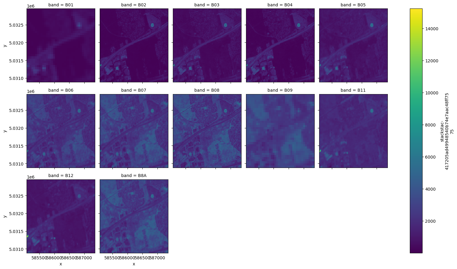
resolution: 10[17]:
# Visualize each band
data[0].plot.imshow(x='x', y='y', col='band', col_wrap=5)
[17]:
<xarray.plot.facetgrid.FacetGrid at 0x7f6de6a84b20>
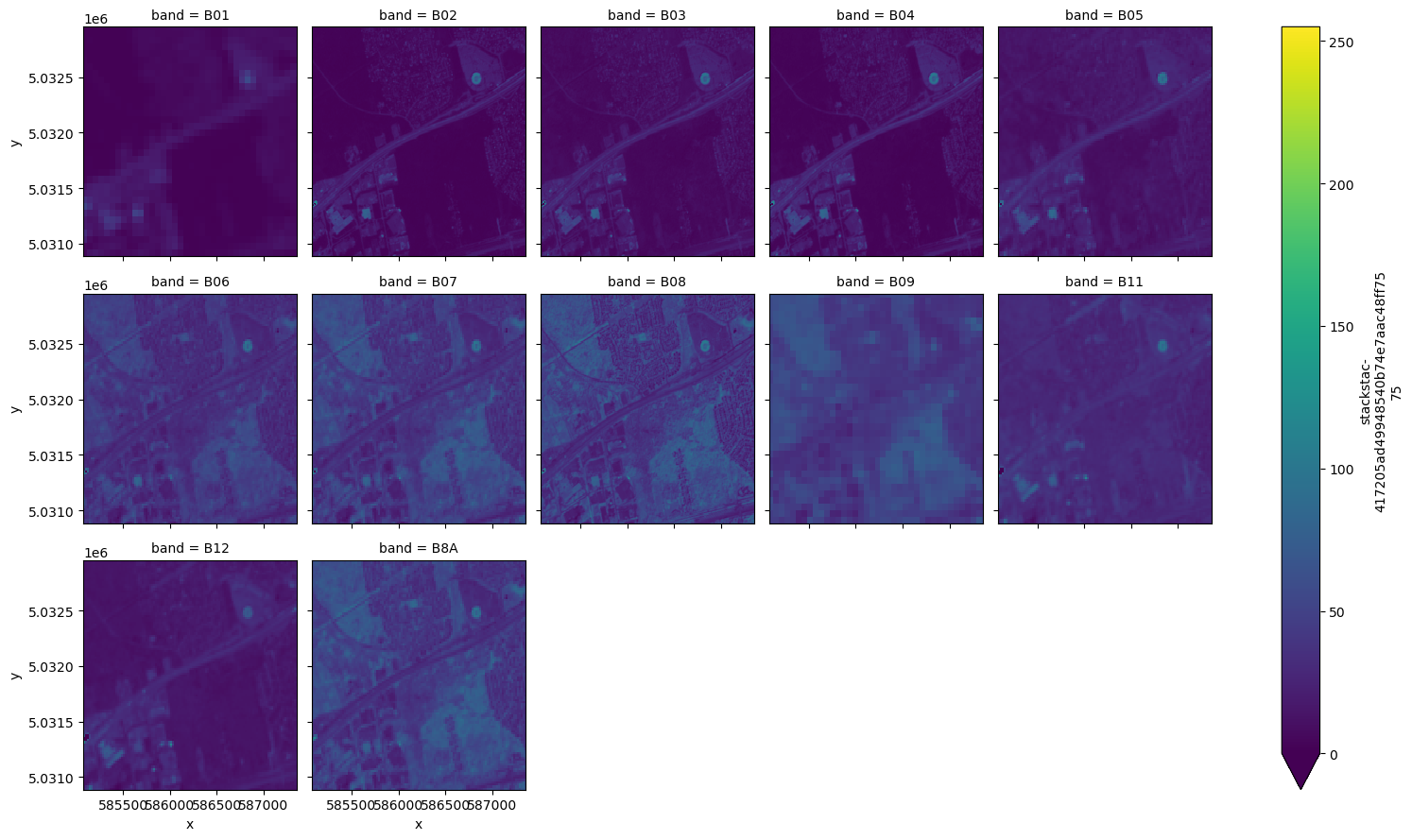
We are going to normalize our data and shift it into a int8 [0, 255] scale.
[18]:
def normalize(array):
    norm = ((array - array.min()) / (array.max() - array.min())*255).astype(np.int8)
    return norm
[19]:
data_norm = normalize(data)
data_norm
[19]:
<xarray.DataArray 'stackstac-417205ad49948540b74e7aac48ff7575' (time: 1,
                                                                band: 12,
                                                                y: 207, x: 228)>
dask.array<astype, shape=(1, 12, 207, 228), dtype=int8, chunksize=(1, 1, 207, 228), chunktype=numpy.ndarray>
Coordinates: (12/44)
  * time                                     (time) datetime64[ns] 2021-08-03...
    id                                       (time) <U54 'S2A_MSIL2A_20210803...
  * band                                     (band) <U3 'B01' 'B02' ... 'B8A'
  * x                                        (x) float64 5.851e+05 ... 5.874e+05
  * y                                        (y) float64 5.033e+06 ... 5.031e+06
    s2:product_uri                           <U65 'S2A_MSIL2A_20210803T154911...
    ...                                       ...
    title                                    (band) <U37 'Band 1 - Coastal ae...
    gsd                                      (band) float64 60.0 10.0 ... 20.0
    common_name                              (band) object 'coastal' ... 'red...
    center_wavelength                        (band) float64 0.443 0.49 ... 0.865
    full_width_half_max                      (band) float64 0.027 ... 0.033
epsg int64 32618[20]:
# Visualize the normalized data and see that it's visually the same as before
data_norm[0].plot.imshow(x='x', y='y', col='band', col_wrap=5, vmin=0, vmax=255)
[20]:
<xarray.plot.facetgrid.FacetGrid at 0x7f6de43faec0>
Initialize K-Means Algorithm#
[21]:
km = dask_ml.cluster.KMeans(n_clusters=4, oversampling_factor=0)
km
[21]:
KMeans(n_clusters=4, oversampling_factor=0)In a Jupyter environment, please rerun this cell to show the HTML representation or trust the notebook.
On GitHub, the HTML representation is unable to render, please try loading this page with nbviewer.org.
KMeans(n_clusters=4, oversampling_factor=0)
Data Preprocessing#
Start by figuring out the shape of our data. Doing so will give us a better understanding of how to manipulate the data for the algorithm.
[22]:
arr_shape = data.shape
arr_shape
[22]:
(1, 12, 207, 228)
The K-Means algorithm requires a 2-dimensional array as an input. First we will essentially flatten the bands invidiually and then we will transpose the array so that each “column” represents a band.
[23]:
arr = data_norm.data[0].reshape(arr_shape[1], arr_shape[2]*arr_shape[3]).T
arr
[23]:
|
||||||||||||||||
Make sure the entire array is visible to the K-Means algorithm (not as chunks - you will get Errors)
[24]:
arr_rc = arr.rechunk({1: arr.shape[1]})
arr_rc
[24]:
|
||||||||||||||||
Fitting The K-Means Algorithm#
Here we will fit our input AOI imagery in to the K-Means algorithm
[25]:
%%time
km.fit(arr_rc)
Found fewer than 4 clusters in init (found 1).
CPU times: user 2.48 s, sys: 105 ms, total: 2.59 s
Wall time: 30.2 s
[25]:
KMeans(n_clusters=4, oversampling_factor=0)In a Jupyter environment, please rerun this cell to show the HTML representation or trust the notebook.
On GitHub, the HTML representation is unable to render, please try loading this page with nbviewer.org.
KMeans(n_clusters=4, oversampling_factor=0)
Predicting Our Classification Clusters#
Once fitted, we can then perform predictions based on the calculated centroids of the input AOI imagery. For simplicity, we are using the same input for both fitting and prediction. Some fitted algorithms can be extended to similar areas - too dissimilar then the results will not be confident.
[26]:
%%time
pred = km.predict(arr_rc)
pred
CPU times: user 22.1 ms, sys: 459 µs, total: 22.6 ms
Wall time: 371 ms
[26]:
|
||||||||||||||||
To visualize the data, we will need to reverse the steps we performed to the input. So, we will transpose and then reshape back into the original X and Y dimensions.
[27]:
pred = pred.T.reshape(arr_shape[2], arr_shape[3])
pred
[27]:
|
||||||||||||||||
Below is an RGB (left) and K-Means Cluster Prediction segmenation map (right) of our input AOI
[28]:
fig, ax = plt.subplots(1, 2, figsize=(20,10))
ax[0].imshow(rescale_intensity(data_norm[0].sel(band=['B04','B03','B02']).data, in_range=(0,30)).transpose(1,2,0))
ax[1].imshow(pred)
[28]:
<matplotlib.image.AxesImage at 0x7f6ddb2aa560>
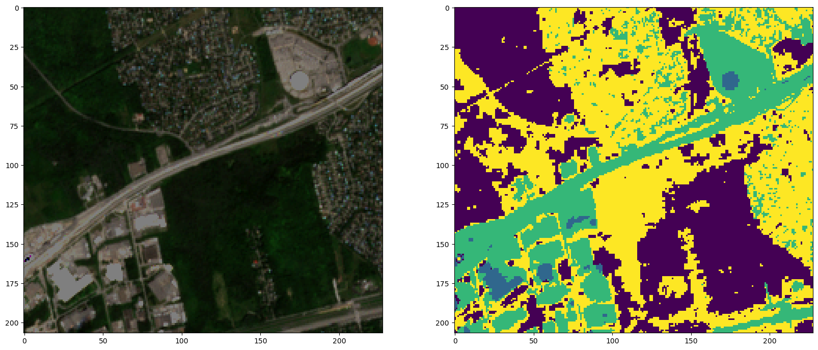
As you can see, the K-Means can easily pick out major concrete infrastructure such as industry areas and highways. It also appears to do a decent job at separating different vegetation densities/types. However, in the residential/urban areas the algorithm doesn’t do as well. That could be an element of the sensor’s spatial resolution and the quality of the segmentation map could be improved on by adding more indicies (eg: NDVI) to the input/prediction operations.