Change Detection

```{admonition} Tutorial does not work on EO4PH Cluster :class: error

This tutorial is specific to the GEOAnalytics cluster deployed to the Google Cloud environment. This tutorial does not work on the EO4PH cluster which is deployed to Azure. ```

Change detection is the process of measuring how the attributes in a particular region have changed over time. Change detection often involves comparing aerial photographs or satellite imagery of the area taken at different times.

Deforestation in Canada

In this notebook we will attempt to identify Deforestation within Canadian forests in Central Ontario, using a naive approach by computing the Normalized Difference Vegetation Index (NDVI). Deforestation is an important issue which results in reduced biodiversity, degrading of soil and water quality, negative wildlife habitat impacts and climate change. Canada covers 9% of all the world’s forests with forests occupying only 38% of Canadian land. Since 1990, thankfully, Canada’s annual deforestation rate has decreased swiftly.

We will be using NDVI (Normalized Difference Vegetation Index) to detect clearcutting in the forests. NDVI values range from -1 to 1, where the higher the value is then the higher amount of vegetation in the area. If there is a drastic decrease over the time period in locations with high vegetation, we can infer it as a deforested area.

There are other ways to identify clearcutting, such as using machine learning algorithms (supervised classification). However, using NDVI takes less computation time while also providing stable results.

The main steps in this tutorial are as follows:

1. Retrieve the satellites images to be used.

2. Compute NDVI using a Dask cluster.

3. Plot the NDVI over time.

4. Create a mask showing the deforested areas within the raster image.

5. Plot the deforested mask on the NDVI mask.

Let’s get started by importing the necessary modules and creating our Dask cluster with 30 workers.

# First initialize the modules
import os
import glob
import re
import datetime
import requests

import rasterio
import dask
import hvplot.xarray

import pandas as pd
import numpy as np
import xarray as xr
import matplotlib.pyplot as plt

from dask_gateway import Gateway
from dask.distributed import wait, progress

gateway = Gateway()

# Cluster configuration
options = gateway.cluster_options()
cluster = gateway.new_cluster(options)

# Scale the cluster
workers = 30
cluster.scale(workers)
# Assign client to this cluster so Dask knows to use it for computations
client = cluster.get_client()

#client.wait_for_workers(workers-3)
cluster

1. Getting the data

We will be using Sentinel-2 Level-2A satellite images for our analysis. The Level-2 products are processed to Bottom Of Atmosphere (BOA) reflectance from the Level 1 Top Of Atmospheric (TOA) reflectance images. These Level 2A images are processed using Sen2Cor which performs the atmospheric-, terrain and cirrus correction of TOA Level 1C data. Using Level 2 images is beneficial since disruptive atmospheric components do not affect the images’ surface reflectance spectra and we do not need to do further image corrections before computation. It is also important to have the lower cloud cover to avoid false negative values when performing analysis on the deforestated data.

If you have completed the NDVI With Dask tutorial notebook, you will notice the same function below is used to get the sentinel data. The only change made is accessing the Level 2 subfolder from the gcp-public-sentinel-2 bucket.

def get_sentinel_data(tile, ron, bands_wanted, months_wanted):
    # 2. Create dataframe to store the path to the granules we want
    df = pd.DataFrame()
    # 3. Get the path of folders, and returns an iterable
    utm = tile[1:3]
    latitude = tile[3]
    direction = tile[4:6]
    dir_path = glob.glob(f'/home/jovyan/gcp-public-data-sentinel-2/L2/tiles/{utm}/{latitude}/{direction}/S2A*{ron}*/GRANULE')

    # 4. Get list of all the files with the wanted bands
    date = 0
    for folder in dir_path:
        band0 = glob.glob(f'{folder}/*/IMG_DATA/R10m/*{bands_wanted[0]}_10m.jp2')
        band1 = glob.glob(f'{folder}/*/IMG_DATA/R10m/*{bands_wanted[1]}_10m.jp2')

        # Check if both files exist
        if not (os.path.isfile(band0[0]) or os.path.isfile(band1[0])):
            continue

        ymd = '\d{4}\d{2}\d{2}' # year, month, day
        get_date = re.search(ymd, band0[0])
        new_date = datetime.datetime.strptime(get_date.group(), '%Y%m%d').date()
        #if image with the same date has already been added, skip
        if (new_date == date):
            continue
        #if image is not from one of the months we want, skip
        if new_date.month not in months_wanted:
            continue
        date = new_date

        #use the path to the GCP url instead of the mounted bucket
        band0[0] = band0[0].replace('/home/jovyan/','https://storage.googleapis.com/')
        band1[0] = band1[0].replace('/home/jovyan/','https://storage.googleapis.com/')

        file_dict = {'date':date, bands_wanted[0]:band0[0], bands_wanted[1]:band1[0]}
        df = df.append(file_dict,ignore_index=True)

    return df

The function parameter ‘T16UDC’ stands for the tile number capturing the region above Lake Superior in Central Ontario, Canada. ‘R026’ represents Relative Orbit Number 26 which covers the entire geographical space in that tile with the highest atmospheric correction. We require the Red and Near-Infrared bands for calculating NDVI, which are Band 4 and Band 8, respectively. The last input parameter is a list of integers for the months to obtain data from, which in our case are June, July, and August.

Images from these summer months are chosen to differentiate between crops and trees when detecting deforestation. Both crops and trees can have high NDVI values, which makes it challenging to distinguish between the two, so a simple way to differentiate the two land-uses is to calculate the mean NDVI value for each of the 3 months through the years. Areas with heavy vegetation - such as coniferous forests - will have high NDVI values for longer than 3 months in a row, while agricultural fields don’t have high NDVI values for long time periods.

%%time
sentinel_df = get_sentinel_data('T16UDC', 'R026', ['B04', 'B08'], [6,7,8])
sentinel_df

CPU times: user 258 ms, sys: 104 ms, total: 361 ms
Wall time: 52.5 s

	B04	B08	date
0	https://storage.googleapis.com/gcp-public-data...	https://storage.googleapis.com/gcp-public-data...	2019-06-03
1	https://storage.googleapis.com/gcp-public-data...	https://storage.googleapis.com/gcp-public-data...	2019-06-13
2	https://storage.googleapis.com/gcp-public-data...	https://storage.googleapis.com/gcp-public-data...	2019-06-23
3	https://storage.googleapis.com/gcp-public-data...	https://storage.googleapis.com/gcp-public-data...	2019-07-03
4	https://storage.googleapis.com/gcp-public-data...	https://storage.googleapis.com/gcp-public-data...	2019-07-13
5	https://storage.googleapis.com/gcp-public-data...	https://storage.googleapis.com/gcp-public-data...	2019-07-23
6	https://storage.googleapis.com/gcp-public-data...	https://storage.googleapis.com/gcp-public-data...	2019-08-02
7	https://storage.googleapis.com/gcp-public-data...	https://storage.googleapis.com/gcp-public-data...	2019-08-12
8	https://storage.googleapis.com/gcp-public-data...	https://storage.googleapis.com/gcp-public-data...	2019-08-22
9	https://storage.googleapis.com/gcp-public-data...	https://storage.googleapis.com/gcp-public-data...	2020-06-07
10	https://storage.googleapis.com/gcp-public-data...	https://storage.googleapis.com/gcp-public-data...	2020-06-17
11	https://storage.googleapis.com/gcp-public-data...	https://storage.googleapis.com/gcp-public-data...	2020-06-27
12	https://storage.googleapis.com/gcp-public-data...	https://storage.googleapis.com/gcp-public-data...	2020-07-07
13	https://storage.googleapis.com/gcp-public-data...	https://storage.googleapis.com/gcp-public-data...	2020-07-17
14	https://storage.googleapis.com/gcp-public-data...	https://storage.googleapis.com/gcp-public-data...	2020-07-27
15	https://storage.googleapis.com/gcp-public-data...	https://storage.googleapis.com/gcp-public-data...	2020-08-06
16	https://storage.googleapis.com/gcp-public-data...	https://storage.googleapis.com/gcp-public-data...	2020-08-16
17	https://storage.googleapis.com/gcp-public-data...	https://storage.googleapis.com/gcp-public-data...	2020-08-26
18	https://storage.googleapis.com/gcp-public-data...	https://storage.googleapis.com/gcp-public-data...	2021-06-02
19	https://storage.googleapis.com/gcp-public-data...	https://storage.googleapis.com/gcp-public-data...	2021-06-12
20	https://storage.googleapis.com/gcp-public-data...	https://storage.googleapis.com/gcp-public-data...	2021-06-22
21	https://storage.googleapis.com/gcp-public-data...	https://storage.googleapis.com/gcp-public-data...	2021-07-02
22	https://storage.googleapis.com/gcp-public-data...	https://storage.googleapis.com/gcp-public-data...	2021-07-12
23	https://storage.googleapis.com/gcp-public-data...	https://storage.googleapis.com/gcp-public-data...	2021-07-22
24	https://storage.googleapis.com/gcp-public-data...	https://storage.googleapis.com/gcp-public-data...	2021-08-01
25	https://storage.googleapis.com/gcp-public-data...	https://storage.googleapis.com/gcp-public-data...	2021-08-11
26	https://storage.googleapis.com/gcp-public-data...	https://storage.googleapis.com/gcp-public-data...	2021-08-21
27	https://storage.googleapis.com/gcp-public-data...	https://storage.googleapis.com/gcp-public-data...	2021-08-31

2. Calculating the NDVI¶

We will be using the same functions and methods from the “NDVI with Dask” tutorial to calculate and output the final Xarray DataArray containing the NDVI of all the raster images. To efficiently get the NDVI for all the data, let’s run the cells below to generate the functions to lazily retrieve the data and output into DataArrays, normalize the data, and calculate the NDVI.

@dask.delayed
def lazy_get_data(B4, B8, chunks={'band': 1, 'x': 12288, 'y': 12288}):
    # Read in the band url as an Xarray DataArray, getting rid of unneccessary dimensions
    red = xr.open_rasterio(B4, chunks=chunks).squeeze().drop(labels='band')
    nir = xr.open_rasterio(B8, chunks=chunks).squeeze().drop(labels='band')

    return (red, nir)

def normalize(array):
    norm = (array - array.min()) / (array.max() - array.min())
    return norm

def get_NDVI(red, nir):

    #Normalize the data
    red_norm = normalize(red)
    nir_norm = normalize(nir)

    # Calculate the NDVI
    ndvi = (nir_norm - red_norm) / (nir_norm + red_norm)

    return ndvi

Now, the code block underneath calls the functions above to load the raster in a Xarray DataArray using a Delayed and get the NDVI of each row from the dataframe created in Part 2. The results from the function call are appended to a list containing the NDVI of every granule.

%%time

# Iteratively load and store the DataArrays for the bands, lazily and append in a list
delayed_ndvi = []
for i,row in sentinel_df.iterrows():
    band = lazy_get_data(row['B04'], row['B08'])
    # Calculate NDVI from the retrieved bands
    delayed_ndvi.append(get_NDVI(band[0], band[1]))

CPU times: user 30.6 ms, sys: 2.39 ms, total: 33 ms
Wall time: 30.9 ms

The next step is to concatenate the list of DataArrays from the previous step with their respective dates into a Xarray DataArray. We will wrap the xr.concat as a dask.delayed decorator function which will be computed, then persisted to the cluster.

delayed_ndvi_concat = dask.delayed(xr.concat)(delayed_ndvi, dim=pd.DatetimeIndex(sentinel_df['date'], name='time'))
delayed_ndvi_concat

Delayed('concat-e4d0c6f4-5aea-4a43-8e0b-5d0a2134f470')

%%time
final_ndvi = delayed_ndvi_concat.compute().persist()
progress(final_ndvi)

CPU times: user 132 ms, sys: 7.65 ms, total: 140 ms
Wall time: 12.4 s

final_ndvi

<xarray.DataArray (time: 28, y: 10980, x: 10980)>
dask.array<concatenate, shape=(28, 10980, 10980), dtype=float64, chunksize=(1, 10980, 10980), chunktype=numpy.ndarray>
Coordinates:
  * y        (y) float64 5.8e+06 5.8e+06 5.8e+06 ... 5.69e+06 5.69e+06 5.69e+06
  * x        (x) float64 4e+05 4e+05 4e+05 ... 5.097e+05 5.097e+05 5.098e+05
  * time     (time) datetime64[ns] 2019-06-03 2019-06-13 ... 2021-08-31

3. Visualizing the Results

Take a look at the hvplot that results from executing the cell below to visualize the change of NDVI in the region over time.

final_ndvi.hvplot.image(groupby='time', x='x',y='y',
                  cmap='RdYlGn', clim=(-1,1), dynamic=True,
                  width=700, height=500)

4. Detecting Deforestation

Once we have our NDVI of the entire region for each date, let’s create a mask showing the deforested areas within the granules.

First, we must rechunk the NDVI Array so the cluster can evenly distribute future Xarray tasks to the workers. Xarray’s .chunk() built-in function chunks based on the partitions on the DataArray dimensions.

scale = len(final_ndvi)//2
chunks = {'time': -1, 'x': int(final_ndvi.shape[1]/scale), 'y': int(final_ndvi.shape[2]/scale)} # chunking into smaller size
NDVI_chunked = final_ndvi.chunk(chunks)
NDVI_chunked

<xarray.DataArray (time: 28, y: 10980, x: 10980)>
dask.array<rechunk-merge, shape=(28, 10980, 10980), dtype=float64, chunksize=(28, 784, 784), chunktype=numpy.ndarray>
Coordinates:
  * y        (y) float64 5.8e+06 5.8e+06 5.8e+06 ... 5.69e+06 5.69e+06 5.69e+06
  * x        (x) float64 4e+05 4e+05 4e+05 ... 5.097e+05 5.097e+05 5.098e+05
  * time     (time) datetime64[ns] 2019-06-03 2019-06-13 ... 2021-08-31

Let’s set our Dask configurations to allow large chunks.

dask.config.set({"array.slicing.split_large_chunks": False})

<dask.config.set at 0x7fba34063850>

Next step is to calculate the mean NDVI values for the months in the year when the alleged forest clearing occurred and compare it with the mean NDVI of the same months in the previous year.

First, let’s group the chunked DataArray by the dates’ year and average according to the year. The computation for this step is done when we want to visualize the data, in Dask. For now it is held lazily.

grouped = NDVI_chunked.groupby('time.year').mean('time')
grouped

<xarray.DataArray (year: 3, y: 10980, x: 10980)>
dask.array<stack, shape=(3, 10980, 10980), dtype=float64, chunksize=(1, 784, 784), chunktype=numpy.ndarray>
Coordinates:
  * y        (y) float64 5.8e+06 5.8e+06 5.8e+06 ... 5.69e+06 5.69e+06 5.69e+06
  * x        (x) float64 4e+05 4e+05 4e+05 ... 5.097e+05 5.097e+05 5.098e+05
  * year     (year) int64 2019 2020 2021

With the DataArray partitioned into years, let’s use the year 2020 as the “After Deforestation” image, and 2019 as the “Before Deforestation” image.

before = grouped.sel(year=2019)
after = grouped.sel(year=2020)

The final step is to create the mask with the non-NULL values highlighting pixels where clear cutting occurred. To detect whether a a forest pixel is clearcut in the following year, we will use Threshold Binarization of the NDVI images. In digital image processing, thresholding is an easy method of segmenting images. If the average of each pixel in the previous year’s NDVI drops by at least 0.25 in the current year, then the pixel is most likely a deforested pixel. The threshold of 0.25 is appropriate for capturing the change in most forest types in the Central Ontario region.

Source: https://eos.com/blog/ndvi-faq-all-you-need-to-know-about-ndvi/

Source: https://www.intechopen.com/chapters/57448

threshold = 0.25

To create the mask, we will be using the built-in xr.where(<condition>, <True>, <False>) function. The condition we will set is if the NDVI average from the current year is lower than the NDVI average of the previous year minus the threshold. If the condition holds true, we will assign the pixel in the mask to 1, and if the condition is false, we assign a NaN.

mask = xr.where(after < before - threshold, 1, np.nan)
mask

<xarray.DataArray (y: 10980, x: 10980)>
dask.array<where, shape=(10980, 10980), dtype=float64, chunksize=(784, 784), chunktype=numpy.ndarray>
Coordinates:
  * y        (y) float64 5.8e+06 5.8e+06 5.8e+06 ... 5.69e+06 5.69e+06 5.69e+06
  * x        (x) float64 4e+05 4e+05 4e+05 ... 5.097e+05 5.097e+05 5.098e+05

5. Plotting the results

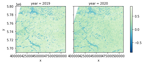
First, let’s show the plots for year 2019 and 2020, our before and after images.

grouped.sel(year=slice(2019, 2020)).plot.imshow('x', 'y', col='year', cmap='GnBu_r')

<xarray.plot.facetgrid.FacetGrid at 0x7fba34154d30>

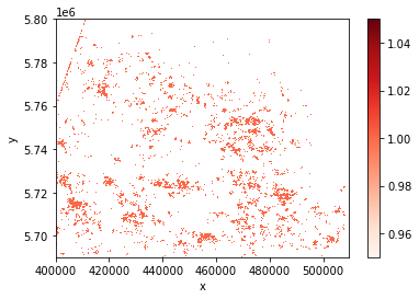
Now, plot to see the resulting deforestation mask we created in the previous step.

mask.plot.imshow(cmap='Reds')

<matplotlib.image.AxesImage at 0x7f7ac6e379a0>

Finally, plot the previous year using the Greys colormap, and overlay the deforestation mask in red.

# Plot forest area from previous year (2019) in grey as a background
plot = before.plot.imshow(cmap='Greys', add_colorbar=False)

# Plot the deforestation mask as overlay
mask.plot.imshow(cmap='Reds',add_colorbar=False,)

plt.title('Forest Loss in Ontario, Canada (2020)');

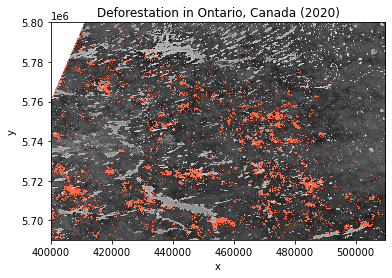
As you can see in the plot above, the red pixels highlight the spots where land cover has changed over the defined period of time. This means that between 2019 and 2020, these forest regions have seen an average drop of 0.25 in NDVI.

Caveat is that it cannot be confirmed that the reason for the forest loss is deforestation. The forest loss could also be caused by wildfires or infestations.

Remember to shut down the cluster!

cluster.close()